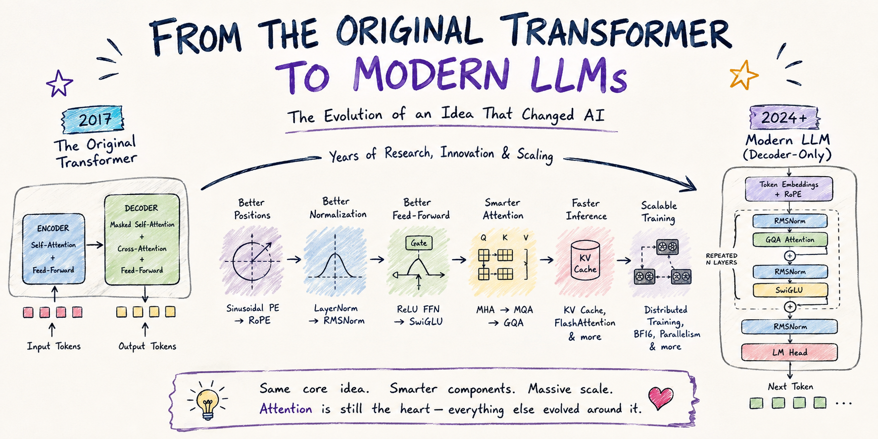
It started with a simple idea.
In 2017, researchers introduced a new neural network architecture in a paper called Attention Is All You Need. They called it the Transformer.
The idea was surprisingly straightforward: instead of processing a sentence strictly from left to right like older recurrent neural networks, a Transformer could look at different parts of a sequence and decide which parts were important to each other.
That mechanism was called attention.
Before going deeper, it helps to understand what a language model actually sees. A model does not directly see words. Text is first broken into small pieces called tokens. A token can be a complete word, part of a word, punctuation, or another small piece of text.
These tokens are then converted into numbers. This representation is called an embedding. An embedding is essentially a list of numbers that allows the neural network to work with the token mathematically.
So, at a very high level:
Text
  ↓
Tokens
  ↓
Embeddings
  ↓
Transformer
  ↓
Output
But there was a problem.
If the model only received the embeddings, it would know which tokens exist, but not necessarily where they appear in the sentence.
Consider:
The dog chased the cat
and:
The cat chased the dog
They contain almost exactly the same words, but their meanings are completely different.
The model therefore needed information about the position of each token.
The original Transformer solved this using positional encoding. Positional encoding adds information about where each token appears in the sequence. The original Transformer used sinusoidal positional encoding, which represented positions using sine and cosine functions.
Now the model had both the content of a token and information about its position.
The next question was the important one:
How does one token know which other tokens matter to it?
This is where self-attention comes in.
Self-attention allows every token to look at other tokens in the same sequence and determine how relevant they are.
Take this sentence:
The animal didn't cross the road because it was tired.
When processing the word "it", the model needs to understand what "it" refers to. Attention gives the model a mechanism for considering other words in the sentence and assigning more importance to the relevant ones.
To calculate attention, the Transformer creates three representations for every token: a Query, a Key, and a Value.
A Query represents what a token is looking for.
A Key represents what information another token can provide.
A Value contains the actual information that gets passed forward when that token is considered relevant.
The model compares Queries with Keys to calculate attention scores. These scores determine how much attention one token should give to another token.
The resulting information is then combined using the Values.
The original Transformer did not use just one attention mechanism. It used several of them in parallel.
These are called attention heads.
Each attention head can learn different relationships between tokens. One head might become useful for nearby words, another might learn relationships between subjects and verbs, and another might capture longer-range relationships.
Using several heads together is called Multi-Head Attention, or MHA.
At this point, the original Transformer block looked roughly like this:
Input
  ↓
Multi-Head Self-Attention
  ↓
Feed-Forward Network
  ↓
Output
The Feed-Forward Network, usually called an FFN, is another neural network inside the Transformer. Attention allows tokens to exchange information with each other, while the FFN processes the information that each token now contains.
The original Transformer used a relatively simple FFN based on the ReLU activation function.
ReLU is an activation function that turns negative values into zero while keeping positive values.
The Transformer also introduced two important pieces that helped it train reliably.
The first was the residual connection.
A residual connection creates a shortcut around a layer. Instead of forcing a layer to completely replace its input, the original information can be added back to the output.
The second was Layer Normalization, commonly called LayerNorm. Normalization keeps the numerical values inside the network in a more manageable range, which makes training more stable.
So an original Transformer block was more accurately:
Input
  ↓
Multi-Head Attention
  ↓
Add & LayerNorm
  ↓
Feed-Forward Network
  ↓
Add & LayerNorm
  ↓
Output
But the original Transformer had something else that is important to understand.
It had an encoder and a decoder.
The encoder's job was to read the input and build a useful representation of it.
The decoder's job was to generate the output.
This made sense for tasks such as machine translation.
For example:
English sentence
       ↓
    Encoder
       ↓
representation
       ↓
    Decoder
       ↓
French sentence
The decoder had its own form of self-attention, but with an important restriction.
It could not look at future tokens.
This is called causal attention, sometimes also called masked attention.
Suppose the model was generating:
I love pizza
When generating "love", it could see "I", but it could not see "pizza".
When generating "pizza", it could see "I love", but not anything after "pizza".
This restriction is essential for autoregressive generation.
Autoregressive simply means generating one token at a time while using the previously generated tokens as context for the next token.
The original decoder also used cross-attention.
Cross-attention allows one sequence to attend to another sequence. In the original Transformer, the decoder could use the representation produced by the encoder while generating its output.
So the original architecture looked roughly like this:
                 Encoder
                    ↓
Input → Self-Attention
                    ↓
             Feed-Forward
                    ↓
                    │
                    ▼
                 Decoder
                    ↓
             Causal Attention
                    ↓
             Cross-Attention
                    ↓
             Feed-Forward
                    ↓
                 Output
This architecture worked extremely well.
But then language modeling started moving in another direction.
Models such as GPT showed that we did not necessarily need both an encoder and a decoder to build powerful language models.
Instead, we could use only the decoder side.
This created the decoder-only Transformer.
A decoder-only Transformer removes the encoder and focuses on predicting the next token.
The training objective becomes beautifully simple:
Given:

"The sky is"

Predict:

"blue"
Then:
"The sky is blue"

Predict the next token.
The model keeps doing this across enormous amounts of text.
This simple next-token prediction objective became one of the foundations of modern Large Language Models, or LLMs.
An LLM, or Large Language Model, is a neural network trained on enormous amounts of text so that it can learn patterns in language and generate new text.
At this point, the Transformer had already changed significantly.
But scaling it up introduced new problems.
The first major problem was positional information.
The original Transformer used sinusoidal positional encoding, but modern language models needed to handle much larger context windows and wanted positional information to interact more naturally with attention.
This led to RoPE, or Rotary Positional Embedding.
Instead of simply adding a positional vector to the token embedding, RoPE applies a rotation to parts of the Query and Key representations based on their positions.
The important idea is that the model can use the relative positions between tokens directly inside the attention mechanism.
So positional encoding evolved from:
Token Embedding
       +
Positional Encoding
toward:
Token Embedding
       ↓
Attention
       ↓
RoPE applied to Q and K
The next problem was normalization.
As models became deeper and larger, training stability became increasingly important.
Modern Transformers often use RMSNorm, or Root Mean Square Normalization, instead of the original LayerNorm.
RMSNorm is a simpler normalization method that focuses on scaling the magnitude of activations rather than performing all the operations used by LayerNorm.
The next major change happened inside the feed-forward network.
The original Transformer used a simple ReLU-based FFN:
Linear
  ↓
ReLU
  ↓
Linear
Modern models commonly use a gated architecture called SwiGLU.
SwiGLU combines the SiLU activation function with a gating mechanism.
A gate is a mechanism that allows one part of a neural network to control how much information from another part should pass through.
The result is a more expressive feed-forward block than the simple ReLU FFN used in the original Transformer.
So now we have something closer to:
Attention
   ↓
RMSNorm
   ↓
SwiGLU
But there was a much bigger problem waiting.
Attention is expensive.
For a sequence containing n tokens, standard self-attention has roughly n² pairwise interactions.
That means the cost grows very quickly as the context becomes longer.
For example:
10 tokens
→ 100 relationships

1,000 tokens
→ 1,000,000 relationships

100,000 tokens
→ 10,000,000,000 relationships
Modern LLMs therefore needed better ways to make attention cheaper.
One important improvement was changing how Query, Key and Value heads are organized.
The original Transformer used Multi-Head Attention, where each attention head had its own Query, Key and Value projections.
Then came Multi-Query Attention, or MQA.
In MQA, multiple Query heads share the same Key and Value heads.
Then came Grouped-Query Attention, or GQA.
GQA sits between MHA and MQA.
Instead of every Query head having its own Key and Value heads, several Query heads share a smaller group of Key and Value heads.
Conceptually:
MHA

Q1 → K1 V1
Q2 → K2 V2
Q3 → K3 V3
Q4 → K4 V4
while GQA might look like:
Q1 ─┐
Q2 ─┘ → K1 V1

Q3 ─┐
Q4 ─┘ → K2 V2
Why does this matter?
Because during generation, Key and Value representations need to be stored.
This brings us to another important modern technique: the KV cache.
KV stands for Key-Value.
When generating text one token at a time, the model does not need to recalculate the Keys and Values of every previous token from scratch.
Instead, it stores them in a cache and reuses them.
For example:
Token 1
  ↓
Calculate K,V
  ↓
Store

Token 2
  ↓
Calculate K,V
  ↓
Store

Token 3
  ↓
Calculate K,V
  ↓
Store
When the next token is generated, the model can reuse the stored information.
This dramatically improves autoregressive generation.
GQA makes this even more attractive because fewer Key and Value heads mean a smaller KV cache.
But attention had another problem.
The mathematical attention operation could be correct while the implementation was still inefficient on GPUs.
This led to techniques such as FlashAttention.
FlashAttention does not fundamentally replace the attention mechanism. Instead, it implements attention in a much more memory-efficient way, reducing unnecessary movement of data between GPU memory and the parts of the GPU performing the calculations.
This distinction is important.
The Transformer architecture can remain conceptually the same while the underlying implementation becomes much faster.
By this point, the Transformer was no longer just a research architecture.
It had become a massive engineering system.
Training modern LLMs requires enormous amounts of computation, so models are usually trained across many GPUs.
A GPU is a processor designed to perform huge numbers of mathematical operations in parallel, which makes it extremely useful for neural networks.
Modern training also commonly uses formats such as BF16, or Brain Floating Point 16. BF16 uses fewer bits than traditional 32-bit floating point numbers, reducing memory and computation requirements while retaining enough numerical range for large-scale neural network training.
But one GPU is nowhere near enough for the largest models.
This is where distributed training comes in.
Distributed training means using multiple machines or GPUs to train the same model.
There are several ways to split the work.
Data parallelism means different GPUs process different batches of training data.
Tensor parallelism means different GPUs handle different pieces of the mathematical operations inside the model.
Pipeline parallelism means different GPUs handle different sections of the model's layers.
There is also gradient checkpointing, a technique that saves memory during training by storing only selected intermediate results and recomputing others when needed.
At this point, it becomes clear that a modern LLM is not simply a Transformer.
It is a Transformer surrounded by a huge amount of systems engineering.
And training is only half of the problem.
Once the model has been trained, we need to run it.
This is called inference.
Inference is the process of using the trained model to generate an output.
Training asks:
How can we update billions of parameters efficiently?
Inference asks:
How can we generate tokens as quickly and cheaply as possible?
That introduced another collection of techniques.
One of them is quantization.
Quantization means representing model numbers using fewer bits.
A model might normally store its parameters using a higher-precision numerical format, but quantization can reduce that precision to save memory and improve inference efficiency.
Other techniques include better batching, optimized GPU kernels, and speculative decoding.
Speculative decoding uses a smaller, faster model to propose several tokens and then lets the larger model verify them. When the predictions are accepted, multiple tokens can effectively be generated with less work from the larger model.
After all these changes, we can finally look at what a modern Transformer block looks like.
A simplified modern decoder-only architecture might look like this:
Input Tokens
     ↓
Token Embeddings
     ↓
RoPE
     ↓
┌────────────────────────────┐
│          RMSNorm           │
│              ↓             │
│       GQA Attention        │
│              ↓             │
│    Residual Connection     │
│              ↓             │
│          RMSNorm           │
│              ↓             │
│           SwiGLU            │
│              ↓             │
│    Residual Connection     │
└────────────────────────────┘
     ↓
Repeat for many layers
     ↓
RMSNorm
     ↓
LM Head
     ↓
Logits
     ↓
Softmax
     ↓
Next Token
The LM Head, or language-model head, converts the model's internal representation into scores for every possible next token.
Those raw scores are called logits.
Softmax converts those scores into probabilities.
For example, after seeing:
"The sky is"
the model might produce something conceptually like:
blue       0.72
clear      0.08
dark       0.04
beautiful  0.02
...
The model selects a token according to its generation strategy, adds that token to the sequence, and repeats the entire process.
And that is the journey from the original Transformer to the modern LLM.
The modern Transformer is not a completely different invention from the one introduced in 2017.
It is the result of years of improvements applied to the same fundamental idea.
The original Transformer gave us attention.
Decoder-only architectures made autoregressive language modeling simple and scalable.
RoPE improved positional information.
RMSNorm simplified normalization.
SwiGLU replaced the simple feed-forward network with a more expressive gated architecture.
GQA reduced the memory cost of attention.
KV caching made autoregressive generation dramatically more efficient.
FlashAttention improved the implementation of attention.
Quantization reduced the cost of running large models.
Distributed training made it possible to train models with billions or even trillions of parameters.
The pieces changed, but the central idea remained remarkably stable:
Let tokens exchange information through attention, transform that information through neural layers, and repeat this process many times.
That is the Transformer.
And the modern LLM is, in many ways, the 2017 Transformer after years of evolution, optimization, and scaling.